Need help with something related to MR physics or protocols? Contact Ross Mair (rmair@fas.harvard.edu).
Available Protocols and Sequences
What are the default scanning protocols used in the center?
Localizer
All our scan sessions begin with a single-slice, three-axis localizer scan that gives a view of the subject’s head in the three scanner-frame axes. In addition, the images from each receive channel are saved separately (uncombined localizer – see below) This lets us check the head coil plugs are all seated correctly and all channels in the coil are working correctly.
AAScout
Takes two low-resolution whole-head scans, and compares the result to a brain atlas on the scanner. This is used to position all future scans in the session, and ensure reproducible positioning if the subject is scanned multiple times. It is very useful, and helps efficiency at the scanner, if you are scanning healthy adults with normal-sized heads, and are obtaining full-brain coverage in your BOLD scans.
If you are scanning children, or patients with neurological disorders, the AAScout may fail completely. If the subject has an overly large head, or you are scanning less-than full brain coverage in your BOLD’s there is a risk that AAScout will not position the slices correctly, and you will certainly want to check the results before continuing, and perhaps manually position slices.
T1-weighted Structural
By default, we use a multi-echo MPRAGE (MEMPRAGE) as this provides a number of benefits over a conventional MPRAGE. The method acquires 4 separate structural scans with different TE values ranging from 1.5 to 7 ms, but in the same time as a conventional scan. This is achieved by using a much higher bandwidth than is usual in an MPRAGE. The higher bandwidth means the image is acquired more quickly and suffers less distortion than an MPRAGE, although image SNR is lower because the wider bandwidth picks up more noise. This SNR deficit is recovered by averaging the 4 separate images together. This results in a structural image with low distortion and high SNR. In addition, because the 4 images have different TE’s, certain areas of the brain are weighted differently in the 4 images and so contrast is different in the resultant average image. This has benefits in automated segmentation of brain structures (as in Freesurfer), and in particular in distinguishing the brain from the surrounding dura. The MEMPRAGE method is described in detail in this reference:
A. J. W. van der Kouwe, T. Benner, D. H. Salat, B. Fischl, Brain morphometry with multiecho MPRAGE, NeuroImage, 40, 559–569 (2008).
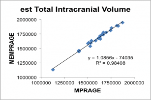
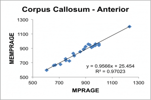
We provide a ~ 6 minute scan with 1 mm3 voxels and two-fold iPAT acceleration, which gives the best-looking images on the screen. A ~ 2 minute scan with 1.2 mm3 voxels and four-fold iPAT acceleration gives a very rapid structural scan that is adequate for automated parcellation/segmentation. We have shown high repeatability of segmentation results for the 2-minute protocol when subjects are scanned multiple times in the same scanner or using different scanners; and have also shown high correlation between the results obtained from the 2-minute protocol and a conventional 6-minute MPRAGE scan.
Below, correlation plots of Intracranial (eTIV) and anterior Corpus Callosum volumes (in mm3) determined for 22 subjects scanned with a 5 min 29 sec conventional MPRAGE and the 2 min 12 sec MEMPRAGE protocols, along with linear regression data.
BOLD
We use a modified BOLD sequence provided by our collaborators at the University of Minnesota Center for Magnetic Resonance Research (CMRR). Their multiband EPI BOLD package provides a large array of advancements over the product Siemens BOLD sequence, including the ability to save out the single-band reference image (useful for checking subject motion and later registration in offline processing), manually control the field-of-view shift parameter for advanced protocols, write out physiological monitoring data into “DICOM” files stored with the image data, as well as featuring an improved and more stable reconstruction algorithm. To help determine appropriate settings for things like TR, slice number, and voxel size please talk to Ross (rmair@fas.harvard.edu)
Diffusion
We use a modified diffusion sequence provided by our collaborators at the University of Minnesota Center for Magnetic Resonance Research (CMRR). Like their multiband EPI BOLD package, their diffusion sequence provides a large array of advancements over the product Siemens BOLD sequence, including the ability to save out the single-band reference image, manually control the field-of-view shift parameter for advanced protocols, control the flip angle of the RF pulses, write out physiological monitoring data into “DICOM” files stored with the image data, as well as featuring an improved and more stable reconstruction algorithm. Anyone interested in using this sequence should contact Ross (rmair@fas.harvard.edu). The basic protocol we provide for standard diffusion MRI has a spatial resolution of 1.7 mm isotropic, 81 slices, 103 gradient directions with b values = 1000, 2000 and 3000 s/mm2, and takes ~ 7.5 min to run, but this can be lengthened or shortened based on your needs.
What other scanning protocols are available in the center?
T2-weighted Structural
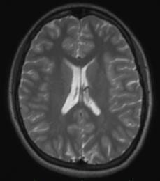
By default, we use a T2SPACE protocol to provide T2 weighted anatomical images. The T2-weighting “reverses” the contrast seen in T1-weighted images, making CSF bright and white-matter dark. An example of a T1– and T2– weighted image from the same subject in the same position is shown below.

Some groups use it in addition to a T1-weighted anatomical scan. The multi-echo MPRAGE (MEMPRAGE) sequence used for T1-weighted anatomical images allows us to match the field-of-view, matrix size and bandwidth of the T1– and T2-weighted images, allowing users to overlay the two or take the signal intensity ratio as an additional diagnostic procedure, as any susceptibility-induced distortion is identical in the two scans. As with the MEMPRAGE, we offer a rapid, lower resolution protocol (1.2 mm isotropic, 2 min 31 sec), and a longer, 1mm-isotropic protocol (4 min 42 sec). Siemens employs a variable-refocusing flip-angle method in the T2SPACE protocol (SPACE stands for Sampling Perfection with Application optimized Contrasts using different flip angle Evolution), and is described in this reference:
M. Lichy, et al., Magnetic resonance imaging of the body trunk using a single-slab, 3-dimensional, T2-weighted turbo-spin-echo sequence with high sampling efficiency (SPACE) for high spatial resolution imaging: initial clinical experiences. Invest. Radiol. 40, 754–760 (2005).
Motion-corrected structural scans
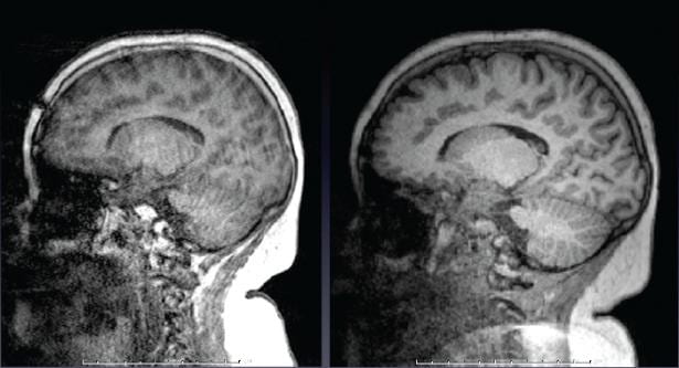
Just like in BOLD scans, subject motion during anatomical scans can be problematical, especially with very young, elderly, or neurologically-impaired subjects, and of course becomes more likely the longer scan is. Therefore, if you want a very-high quality anatomical scan and so run a longer scan with higher spatial resolution and less image acceleration, the likelihood of motion corrupting the scan becomes higher too. Motion in anatomical scans can result in blurring or ringing in the image. Our collaborators at MGH have devised a method where a very rapid, very low resolution, 3-D scan can be acquired and analyzed in ~ 250 ms – which is less time than the T1-weighting period (TI) usually employed in MEMPRAGE scans. The low-resolution 3D navigator image is then assessed for motion since the previous navigator, and the field-of-view/slice positioning for the anatomical scan is updated in real time during the anatomical scan. Additionally, they provide a method for the scanner to determine the slices in the anatomical scan most corrupted by motion, discard then and re-acquire them. The number of slices to be reacquired is set by the user – this adds some time to the scan, but the results can be impressive. The example below (c/- Children’s Hospital, Boston) shows a T1-weighted image of an unsedated child, without motion correction on the left, and with motion correction on the right.
The exact same image protocols described above for T1– and T2-weighting are available with motion correction as well. We recommend nearly every one use these motion-corrected anatomical scans. Especially if you are scanning young or elderly subjects, or those with neurological disorders, this is a good idea. Contact Ross (rmair@fas.harvard.edu) if you want to employ these scans, as there are some tricks to the set-up and running of them. The motion-correction method is described in detail in this reference:
M.D. Tisdall, et al., Volumetric Navigators for Prospective Motion Correction and Selective Reacquisition in Neuroanatomical MRI. Magn. Reson. Med., 68, 389-399 (2012).
Motion-Corrected BOLD (PACE)
PACE is a Siemens term for employing prospective motion correction to BOLD scans. (PACE is an acronym meaning Prospective Acquisition CorrEction.) The concept is very similar to the motion-corrected anatomical scans as described above, however this time additional navigator scans are not needed. Instead, the scanner compares the 3D volumes acquired in the first and second time-points of the BOLD scan, determines what (if any) motion has occurred in that time, and then updates the position of the field-of-view and slice alignment before the third time-point is acquired. This continues throughout the scan, with the image position for each time-point updated based on motion correction parameters calculated from the previous two time-points. Although Siemens offers a product PACE sequence, we use a modified PACE sequence provided by our collaborators at the Martinos Center at MGH. ep2d-pace-MGH provides the same additional features to the product PACE sequence as ep2d-BOLD-MGH does – mainly the ability for the user to set a pre-defined number of dummy scans.
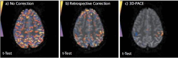
Opinions vary on the usefulness of PACE. Some users swear by it, saying it allows them to recover BOLD activations they would not otherwise see even after offline motion correction. Others prefer not to have the scanner changing anything during their BOLD scans, especially as the “uncorrected” data is not available. Some also feel the time-lag for correction (which is two TR’s, or up to 6 seconds or more) is too long, and that by the time the motion correction has been calculated and applied, the subject may no longer be in the same position. By its very nature, the PACE method is best at dealing with slow coherent motion, such as the subject’s head slowly sinking further into the pillow over time, or scanner drift; while if a subject undergoes a sudden jerky motion (eg., sneezes) and then returns to their original position, it might take the scanner 4 or 5 TR’s to catch up with that motion. That said, some of our users most keen on PACE are those who scan children, so they certainly see benefit in the method despite the potential drawbacks. In the Center, we don’t make a specific recommendation on whether you should use PACE or regular BOLD, however Ross (rmair@fas.harvard.edu) will gladly discuss your specific case with you. As the PACE scan is essentially a BOLD scan with additional processing, any BOLD scan protocol that successfully runs on our scanner (TR, spatial resolution, number of slices) can be converted to a PACE protocol. The figure below (taken from a Siemens brochure, so it’s a “best case scenario”), shows BOLD activations from a PACE scan (right), and comparably thresholded data from a traditional BOLD scan (left) and that scan just with retrospective motion correction – or the equivalent of offline motion correction (middle). The subject was instructed to move their head slightly throughout the experiment.
Field Mapping
A field-mapping scan enables offline distortion correction of your BOLD images during post-processing with software such as SPM or FSL. The field-map scan acquires two simple T2*-weighted images using the gradient echo method. T2*-weighting is similar to the T2 weighting described above, except that the signal is more heavily weighted by effects from susceptibility-induced gradients (drop-out as well as distortion). The two images are acquired with different TE times, to produce different weightings. A simple formula relates the phase-difference of the signal in each voxel to the 3D field variation in that voxel. The offline processing software can then figure out how much to “un-distort” each voxel based on the field variation in that voxel.
Talk with Ross (rmair@fas.harvard.edu) if you want to add this feature to your scanning protocol. The scan must be set up with the same field-of-view, spatial resolution and number of slices as your BOLD scan, so if you vary these parameters, a field-map scan will need to be set up for each one. For most common BOLD scan parameters, the field-map scan takes about a minute. As with other methods described above that rely on pre-scans of any sort, subject motion works to invalidate any correction, so these methods are really only useful for very compliant subjects that can remain still for extended periods. The reference for this method is:
P. Jezzard, R. Balaban, Correction for geometric distortion in echo planar images from B0 field variations. Magn. Reson. Med. 34, 65–73 (1995).
Arterial Spin Labeling (ASL)
ASL is a variant of the BOLD scanning method, that enables quantification of blood flow to different regions of brain. This is done by saturating or preferential exciting blood while it is still in the arteries below the brain, and then measuring changes in the brain signal level after some time has elapsed. ASL is still something of a method-under-development. There are a variety of methods by which the general concept can be implemented – they have a variety of acronyms for names and all have pros and cons. The method was have available on our scanner is a “pseudo-continuous ASL” (pc-ASL) method, coded for Siemens scanners by folks at Univeristy of Pennsylvania. Derivation of the blood flow map needs to be done offline and will not happen on the scanner. As of February 2013, no-one has employed this technique in a study here at Harvard. However, feel free to contact Ross (rmair@fas.harvard.edu) if you think this technique may be of interest to you. The reference for this method is:
W. Wu, M. Fernandez-Seara, J. Detre, F. Wehrli and J. Wang, A Theoretical and Experimental Investigation of the Tagging Efficiency of Pseudocontinuous Arterial Spin Labeling. Magn. Reson. Med. 58, 1020-1027 (2007).
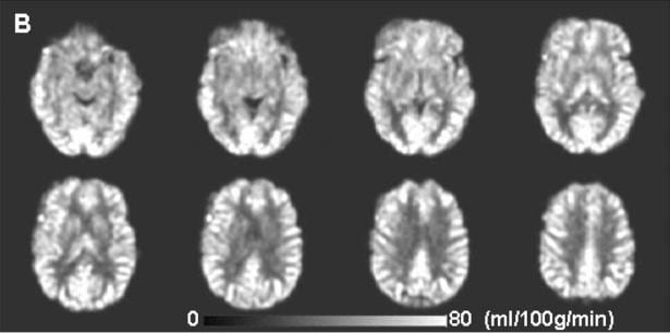
The images below show an example of the quantitative images of cerebral blood flow obtained with pc-ASL (from Xu et al, NMR Biomed. 23, 286-293 (2010)).
Are there special sequences to improve/monitor data quality?
Uncombined Localizer
This scan runs exactly the same sequence on the scanner as the traditional localizer – namely a central slice view of the subject’s head in the three scanner-frame axes. However, for diagnostic reasons, we make the scanner display the image from each receive channel on the head array coils we use. For the 12-channel coil, you’ll usually get 4 images per slice; while with the 32-channel coil, you’ll get 32 images. This display allows you to quickly check that everything is OK with all parts of the coil, and that you’re not losing any signal because of bad elements or plug connections. This should not happen, and we’ve never had problems with the 12-channel coil. However, in 2012, we had two different problems with the 32-channel coil. Given the engineering complexity of both the 32-channel coil and the receiver pathway hardware, we now strongly advise all groups using the 32-channel coil to use this localizer scan and check the results before getting too far into your session. It’s a good idea for 12-channel coil users to run this scan also.
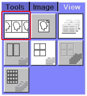
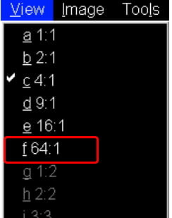
The easiest way to view the results is to go to the Viewing task card, and put the viewing display into stripe mode, so that all images from one series are displayed in adjoining image windows. You can do this with the Stripe button on the right side of the viewing task card. (The default setting is stack mode, which shows each series in adjoining windows – the button for this is next to the stripe mode button.) Once the viewer is in stripe mode, you can choose the 16:1 window display button, or (for the 32-channel coil) choose 64:1 from the View pull-down menu. (64:1 is only available if stripe mode has already been chosen.)
The examples below focus on the 32-channel coil. In the 64:1 view mode, you’ll see the images from the 32 receive channels for the sagittal and coronal view. If you scroll further, or use the slide bar on the right of the image display, you’ll then see the 32 images for the axial view. The example below shows the coronal and axial views.
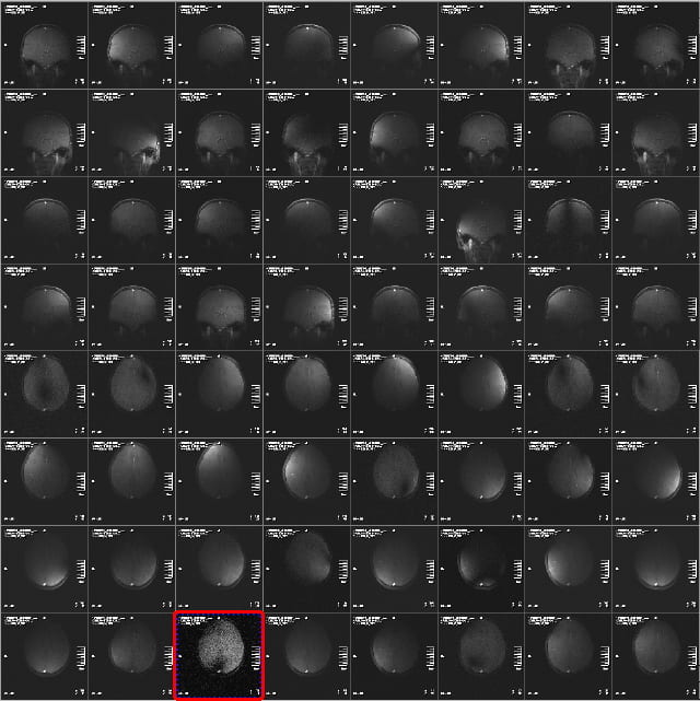
The signal intensity in the images from the different receive channel will vary a lot, and will often only show portions of the brain, or portions of it with “holes” or dark stripes through it. This is normal, as the different receive coil elements are designed to give a smooth, uniform image when added together. Especially in the axial view, its common to see a few elements with low signal (highlighted above), because the coil elements around the crown of the head are a long way from the pure axial slice. You’ll notice however, that the corresponding images in the sagittal or coronal views have high signal. This, therefore, is what you want to see – it indicates the coil as working properly.
Problems are indicated by seeing little or no signal in a few channels, and having the same problem in the same channels in the different views. Two examples are shown below, where the signal is non-existent, or has pixel values of 0 and 1 only, but there is no background noise – and the result is the same in two views (and was the same in the third view).
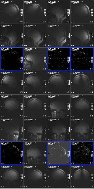
This indicates a problem with the plug or the socket it plugs into. Siemens replaced the sockets on the patient table in 2012, and so this problem has, at this time, been mostly eliminated. However, its still possible to insert plug #3 (closest to front of magnet, left side, if viewed from the front of the bore) enough for the scanner to believe it is plugged in correctly, but for the plug to not be fully seated in the socket. If you see this problem, slide the patient table out, and unplug and replug your coil plugs (and let Ross (rmair@fas.harvard.edu) know).
The other problem experienced in 2012 was two elements ceasing to function on the coil. This could have been due to problems with the electrical connections in the coil elements themselves, or the electrical components on the coil body that those elements were connected to. In this case, the symptoms were images from those elements showing bright fuzzy noise, but with no image data whatsoever. Again, the same problem is seen in all three views, not just one slice. And in this case, the problem is seen repeatedly each time the coil is used. Re-plugging won’t help – the coil was replaced. If you believe you are seeing anything like this, let Ross (rmair@fas.harvard.edu) know.
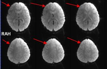
There is much redundancy in the coil design, so even if a few elements are not working correctly, it may be hard to see any impact on your structural or BOLD scans. The figure below shows a BOLD scan acquired when 5 coil elements were not recording any signal, due to the plug/socket problem described above, The signal in the BOLD scans is lower on the left side of the slices than the right. The brain can still be seen, and perhaps the data is still usable as the effect is constant throughout the scan. However, given we do everything else to get maximal signal from the brain with a $3 million scanner and a $100,000 head coil, its worth taking a minute or two to check its all working for you as it should!
What is iPAT?
iPAT is the term Siemens uses for its parallel imaging implementation. It stands for integrated parallel imaging techniques and is the general term for the entire family of receiver coil-based data acceleration methods. When using parallel imaging methods, spatial information is partly acquired from the receive-field of the RF coil elements, and partly from k-space (i.e. gradient) encoding. By comparison, with conventional, non-parallel imaging we only use k-space encoding. Using iPAT means that we can acquire fewer gradient echoes and so acquire less data per volume during an EPI time series. The iPAT number refers to the image acceleration factor – or in the case of EPI, the reduction in the length of the echo train. For example, with iPAT = 2 we acquire half of the number of echoes for EPI as without iPAT, while with iPAT=4 we would acquire only one quarter of the gradient-encoded data than would be needed without iPAT. There are two flavors of iPAT available for nearly all sequences on the scanner: GRAPPA (“generalized autocalibrating partially parallel acquisitions”) which is k-space-domain based, and mSENSE (“modified sensitivity encoding”) which is image-space based. GRAPPA is recommended by Siemens on their scanners and has been shown to be better than mSENSE for fMRI, so this is what we use. You do have a choice of how much acceleration you want to have, such as a factor of 2, 3, or 4. iPAT =1 means iPAT is turned off.
So what happens if you have GRAPPA enabled? Well, in exchange for being able to skip k-space lines in each EPI, we need to map spatial information at the start of the acquisition. With iPAT=2, two reference EPI volumes are acquired. These happen immediately after dummy scans and before the first real (saved) volume of EPI. (Higher iPAT factors require more reference steps, in proportion.) Not only do these reference scans add some time to the total measurement, but of more importance is that it is essential there be no subject motion while they are acquired! If the subject moves during those critical few seconds – for iPAT=2 and TR=2000 ms the reference scans would take 4 seconds to acquire – the spatial reconstruction will be affected, causing all of the EPIs in the subsequent time series to have artifacts in them.
How do you know if your subject moved during these reference acquisitions? Well, all you can do is open the Inline Display window as soon as you’ve started the scan and wait to see the EPIs that result. If the subject did move during the reference scans, you’ll see artifacts in the images and these will stay fairly constant as the scan progresses. Contrast this with a situation where the subject does NOT move during the reference scans, but does move a short time thereafter. In this case, the EPIs will start out looking pretty good, then occasionally go bad with the subject movement, then perhaps go back to looking good again, etc. In summary, then, if the images start bad and stay bad, bet that the subject moved during the GRAPPA reference acquisitions and stop the scan. Remind the subject to lie as still as possible, and start again.
One related trick is to ask the subject to swallow before the scan starts, and ask him not to swallow again until he has counted to ten seconds after the start of the EPI noise. With a TR of 2 seconds and two dummy scans the subject won’t then swallow until after the third real volume of EPI is being acquired. (Recall 4 secs of dummy scans, 4 secs of reference acquisitions for iPAT=2, then the first real EPI volume is acquired.) Many subjects don’t consider swallowing (or moving their eyes come to that!) as ‘head’ movement. Politely remind them that at the beginning of the scan it is also important to keep everything still, including the eyes, the mouth/throat, arms, and legs).
Is iPAT/GRAPPA a good technique to use? What are the caveats?
In general, the decision whether or not to use iPAT (GRAPPA) – is driven by the spatio-temporal requirements of your experiment. If you can meet your voxel resolution and spatial coverage (slices per TR) requirements without GRAPPA, then do so. Adding GRAPPA will translate into additional motion sensitivity in your BOLD scans. You will only want to consider GRAPPA if you need higher spatio-temporal resolution than can be achieved with full k-space EPI. The reduction in the echo train length – by a factor of 2 for iPAT =2, etc – does help to reduce signal distortion and drop-out, due to the effects of susceptibility gradients as described below.
If your main region of interest is a high-susceptibility area, you might opt to use iPAT with the express purpose of reducing distortion/drop-out. However, in general we would not recommend this, as the potential for motion artifacts and reduced SNR will probably outweigh the gains.
What about the caveats of using GRAPPA? First of all, you never get something for nothing! GRAPPA reduces SNR, even in the absence of motion. Sampling a shortened echo train with iPAT=2 reduces the image SNR by √2, or 40%. Next, there may be artifacts in the reconstruction process caused by the mixture of imperfect receive-field encoding with a k-space encoding process. These reconstruction errors tend to increase with increasing iPAT factor and are decreased as the number of RF coil elements gets larger. This is essentially why we can’t use higher than iPAT=2 with the 12-channel coil; we need more channels (coil elements) to push up to iPAT=3 or 4. We are currently in the process of investigating what the implications of iPAT might be on measures such as t-stats, % signal change, and tSNR).
What is “partial Fourier” and why might I want to consider it for EPI?
Partial Fourier (pF) is another approach to reducing the number of k-space lines acquired in order to produce an echo planar image. (It can also be used for non-EPI sequences but here we will focus on its use for EPI.) Like parallel imaging methods, pF is intended to speed up data acquisition, usually as a way to increase the spatio-temporal resolution. However, unlike parallel imaging techniques such as GRAPPA, pF doesn’t require any sort of reference scan; all the information needed to reconstruct a particular EPI slice is contained in that (partial) slice acquisition. Rather than acquiring every single echo in the EPI echo train, in pF acquisitions just over half of the echoes are acquired by omitting usually ¼ or 3/8 of the phase-encoded echoes in the train. This allows the TE to be shortened, thereby allowing more slices per unit time. To reconstruct the final EPI from a 2D FT we need to synthesize the missing k-space lines. This is permissible because k-space of a real object, such as a brain, exhibits a symmetry provided certain conditions are met. The high k-space lines sampled in the first half of the acquisition can be converted mathematically into the missing lines in the second half, albeit with a slight reduction of the SNR for these lines. (By sampling only once their SNR is reduced by √2.) Then, once a complete k-space matrix has been obtained, the resultant can be 2D Fourier transformed to yield images).
Is partial Fourier a good technique to use? What are the caveats?
In general, partial Fourier should only be considered when you wish to use a TE that is considerably shorter than can be attained by the acquisition of your desired full k-space matrix. You might want to have a shorter TE to reduce dropout, and/or to increase the amount of spatial coverage (i.e. slices per TR). Assume you want to end up with images that are 128×128 pixels, and full k-space coverage requires a minimum TE of 44 ms. But you want to use a TE of 30 ms for optimal BOLD signal, and because shaving 14 ms off the acquisition time for each slice is needed to get sufficient brain coverage in the slice dimension, given your required TR. By omitting the first thirty-two of 128 echoes (i.e. using 6/8ths partial Fourier) it is possible to reduce the minimum allowable TE by ~ 16 ms, thus allowing the desired TE of 30 ms. You will acquire only 96 x 128 data points while the scanner will reconstruct the “missing” 32 lines of data in the phase encode dimension to yield the desired images of 128×128 pixels.
There are of course caveats to partial Fourier scanning. In synthesizing the omitted k-space it is necessary in the reconstruction process to estimate the phase of the computed data. The phase of the acquired k-space lines on the fully sampled half of k-space isn’t appropriate for the synthetic lines. Regional variations in resonance frequency, i.e. shim imperfections, lead to different phases for k-space lines acquired at different times after the excitation RF pulse, so the late (acquired) echoes will necessarily have different phase than the early (omitted) echoes. This is why some echoes (32 in the example) are acquired in both halves of k-space. If we were to acquire only 4/8ths of k-space – just one half – it would be difficult to get the phase of the omitted half correct, and artifacts would result. By acquiring at least 2/8ths of k-space in each half, smooth phase can be assured and artifacts are minimized. (Note that Siemens allows only 6/8ths or 7/8ths partial Fourier sampling for EPI.)
Another caveat is image SNR and signal drop-out. By acquiring only 6/8ths of the echoes in a full echo train, the per image SNR is decreased by sqrt(8/6), or 15%, compared to the full 8/8ths sampling. Additionally, not all signal regions in every EPI slice will refocus at exactly the center of k-space. Well-shimmed regions, especially in occipital and parietal cortex, will likely refocus at kx,y=0, and so should obey the SNR rules just mentioned. But regions suffering from strong magnetic field gradients – the usual suspects of frontal cortex and lateral temporal lobes – may refocus earlier than the theoretical center of k-space, resulting in increased signal dropout).
It looks like I will need to use either partial Fourier or iPAT to get the spatial resolution and coverage that I want. Which method should I use?
An obvious question, given the need to reduce the minimum attainable TE and/or increase spatial coverage (in terms of slices/TR), is whether to use GRAPPA or partial Fourier. There is no simple answer to this question, but there are a handful of points to consider. The first is your intended use. If you want to shorten the minimum attainable TE and can achieve the TE you want using partial Fourier, then that is probably a good enough reason to stick to pF; it doesn’t require any form of “reference scan” so it has lower motion sensitivity than GRAPPA. However, unlike GRAPPA, using partial Fourier does not reduce the level of distortion inherent in the phase-encoded dimension of the EPIs. Thus, if one of your intentions is to reduce distortion you might want to use GRAPPA and the highest acceleration factor that your experiment can tolerate subject to the reduction of SNR, the presence of residual aliasing artifacts, the enhanced motion sensitivity and all the other fun stuff that comes with that method! But do not despair! By the time you are ready to consider partial Fourier or GRAPPA for your protocol, it is time to talk to Ross (rmair@fas.harvard.edu) for an in-depth discussion of your experiment).
At the scanner
When does shimming happen and what is actually done?
Shimming is the term given to the optimization of the magnetic field over the subject’s brain. In the absence of a subject, the magnetic field is homogeneous to a few parts per million across a 30 cm diameter spherical volume (DSV). But the subject’s head degrades the field considerably. Because air, bone, tissue, etc. all interact with an applied magnetic field in different ways, spatially complex magnetic field gradients (susceptibility gradients) are established at the interfaces between different tissue types. In places, like across the frontal lobe, the field heterogeneity can become as bad as parts per hundred. Unless this degradation is accounted for, echo planar images (or those regions of EPIs where the field is most heterogeneous) may have low signal (i.e. “dropout”), high distortion and high artifact (ghost) levels.
To compensate for this degradation of the magnetic field, the “bad” field regions are opposed (and ideally cancelled) by small magnetic fields generated by resistive (copper) coils that are wound on the gradient set, inside the magnet bore tube. You don’t really need to know anything about these coils, other than that they exist. Unless otherwise instructed the scanner will perform shimming automatically using a field mapping procedure, over a volume that encompasses your slices/volume of interest. No further shimming will be conducted in the current scan session unless you request a re-shim explicitly. In general you’ll find that you’ll get a shim based on either your first EPI prescription or your MPRAGE, whichever comes first in your protocol, and that’ll be it for the session. The shimming routine involves a magnetic field map acquisition. This is a 20 second buzzing that happens before the scan you’ve just initiated. The scanner acquires this field map and computes a correction based on the result. Expect the 20 seconds of buzzing only for the first EPI (or your MPRAGE) scan in your protocol. After that, the only noise you’ll hear before your EPI starts is a couple of quick clicks.
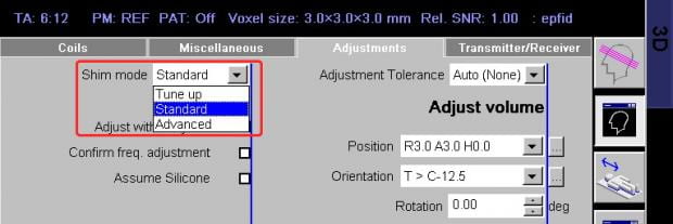
An advanced shim mode is available. In this mode, the scan does a first field map as in the standard mode and then acquires a second map to check the validity of the first. A small correction is made, if necessary, and a third field map is acquired to check that result. The total advanced shim takes approximately 90 seconds, whereas the standard shim takes 30 seconds (including computations).
Should you use standard or advanced shimming? Well, based on the appearance of EPI ghosts, it seems that standard shimming is perfectly acceptable. You probably won’t see any visible differences in EPI quality if you compared the two methods by eye, but you might find small improvements in fMRI statistics in hard-to-shim areas like frontal lobe. If you have the time in your protocol, and are interested in partial brain coverage (e.g. occipital-only, or frontal-only scans), or hard-to-shim areas, it might be worth a try.
Finally, it is also possible to change the volume over which shimming is performed. The default shim volume is set to cover the entire 3D volume of your slice prescription (either the MPRAGE or EPI, whichever happens first in the imaging session). However, sometimes a user-defined shim volume (usually smaller) can be useful if you are trying to do fMRI of a restricted volume such as the amygdala, LGN or occipital pole. Please contact Ross (rmair@fas.harvard.edu) if you might be interested in this.
How can I make the scanner shim more often?
If your subject has been moving throughout your BOLD scans, despite your exhortations to them not to, you may start to see more numerous or more intense artifacts in the BOLD images – especially ghosts. As the scanner has shimmed the field before the first BOLD scan to make it as uniform as possible, if the subject has moved since that time, the field uniformity has been degraded. Ghosts may increase, and dropout or distortion may be more prevalent as well. In these cases, it is good to know how to make the scanner shim again before the next BOLD scan. An additional 20-30 seconds might help your data quality considerably, and is a lot quicker than trying to figure out why the ghost levels may have increased. Here’s how to make the scanner shim again at any time during a session:
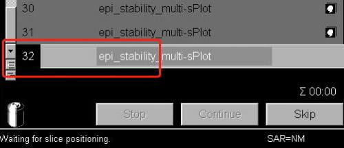
- Ensure the scanner is not already running or that you have other scans that are queued, ready to run automatically before the scan you want to shim for.
- In the exam window (where you start/stop scans) open the next scan (i.e. the scan you’re about to run). The scan number in the queue will go black. Doing this also shows the slice prescription in yellow on the three image display windows.
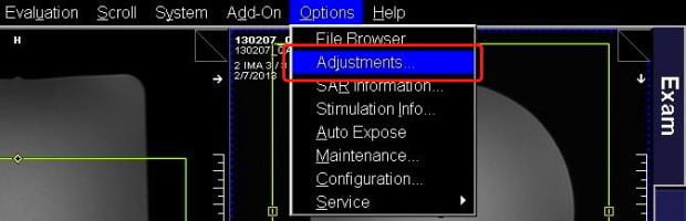
- Now that the current protocol is open, select Adjustments from the Options pull-down menu at the top right of the screen.
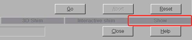
- The very large Manual Adjustments window opens. Ignore everything on here except the tab labeled Show towards the bottom-right. It’s the last in a row of five tabs. Click on this.
- On the Show tab, you’ll see the current shim values in the middle of the window. Again, there’s no need to worry about anything here except the Invalidate All button on the left side. Click this.
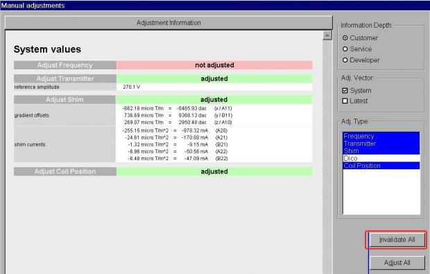
- You’ll now see all the prior shim values have been erased. Just click Close at the bottom right to close the Manual Adjustments window.
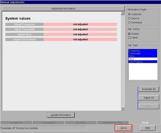
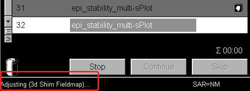
- Now start your scan as normal, using the Apply button above the protocol window. You should see a message in the bottom-left corner of the screen telling you the scanner is redoing its frequency and transmitter adjustments (very quickly), and then that its shimming.
You can repeat this process any time during the session. If you are running very long BOLD scans (> 5 mins) with very little gap between scans (> 30 seconds), it is also useful to re-shim after 1 or 2 BOLD scans to mitigate heating effects in the gradient coils and the passive shims (metal rods inserted in the gradient coil when the coil is installed).
Note, however, that if you are using a field map for offline distortion correction, or the inline distortion-unwarping sequence, you’ll need to acquire a new field map or distortion pre-scan each time you shim.
What is a ghost in EPI images?
The EPI pulse sequence is a train of gradient echoes, with each echo encoding a piece of the second image dimension, the phase-encoded dimension. To make the acquisition faster, we acquire every second echo in the alternate direction through k-space – in effect, time travels forwards for the odd-numbered echoes but backwards for the even-numbered echoes. Before the images you look at can be reconstructed with a 2D Fourier transform, the even-numbered echoes must first be time-reversed, so all echoes are consistent with each other before the 2D FT.
This is a relatively trivial processing step, however there is a catch. Any effect that causes the acquisition of the two echoes to not be a perfect mirror-images of each other will cause problems. Imagine there is a simple delay at the very start of the gradient echo train. From the standpoint of the data in the echo train, this looks like a delay at the start of the sampling period for the odd echoes but a delay at the end of the sampling period for the even echoes! The delay manifests itself in a zigzag manner across the entire set of gradient echoes. The zigzag delay causes a different phase for the odd and even echoes – the phase zigzags in proportion to the delay – and when we then apply the 2D FT that phase zigzag creates an ambiguity in the spatial position of the brain signal. In fact, the ambiguity is at exactly half the field-of-view and is effectively a violation of the Nyquist sampling theorem.
For this reason these ghosts are often called Nyquist ghosts or N/2 ghosts, where N refers to the field-of-view. The bigger the delay, the bigger the phase zigzag, the more the signal is deposited at the half field-of-view position instead of the correct spatial position. Below is an example of a ghosted EPI:
In the above example it was necessary to increase the image intensity quite a lot to visualize the ghosts. That is typical for a well-shimmed, low ghost EPI. As a rough rule of thumb – and given that it is difficult to estimate on-the-fly, by inspection – the ghost level should be 5% or less than the intensity of the brain signal
What are some physical causes of the phase zigzags that lead to Nyquist ghosts? In short, any physical effect that causes a temporal mismatch of the data sampling periods (i.e. when the analog-to-digital converter is turned on) and the readout gradient waveform will lead to ghosts. Poor shimming, and anything that degrades the shim – such as subject motion over time – are often a key cause. Longer echo trains amplify this problem, and so have more noticeable ghosts than short echo train experiments. As a result, lowering the phase-encode resolution or using parallel imaging acceleration can reduce the ghosts.
Another offender is the oblique (slice) angle of the field-of-view. Each physical gradient (Gx, Gy or Gz) has a slightly different electrical inductance and thus has a different response rate to being switched on/off. When the readout and phase-encode axes are “mixed” in the magnet reference frame by an oblique slice angle, the read and phase encode gradients employ a mix of physical gradients. This leads to a difference in the rate at which one component of the gradient pulse comes on compared to the other component – which will also produce the phase zigzags described above. The easiest way to get rid of this is to try rotating your slices slightly, either more or less oblique.
To see what kind of ghosting you are getting and whether it improves, you can run a short test BOLD EPI with just a few timepoints (i.e. 5), and view them to assess the situation before you collect all your data and then realize something didn’t look good. )
What if my ghosts are fluctuating?
As explained above, ghosts are generally a fact of life in the EPI scans used for BOLD studies. What we hope to see is that the ghosts, if present, are very low level, and that they are consistent across time-points. If this is not the case, then something is wrong, and if the ghosts are bright and covering a substantial section of the brain, your data could be compromised. What might cause the ghosts to change during your experiment?
Motion: The most likely cause is subject motion. If the subject readjusts their position on the patient table, their head will move inside the coil. This movement will disrupt the uniform magnetic field created by the shimming process, and so the ghost level will likely increase. However, if the subject just moves once, and then remains in their new position, the ghost level will probably remain constant after the motion, just at a higher level than before. If you detect this in the inline-display window, you can re-shim before the next scan in your session.
Image Reconstruction: If the ghosts are fluctuating rapidly from time-point to time-point in just a few slices, you might be experiencing a problem with the Siemens image reconstruction method. The default method of image reconstruction on the Trio employed a constant zero-order phase correction to all the k-space data, however we (and other sites) noticed as the 32-channel coil was more commonly used, that this correction would sometimes fail, resulting in large, intermittent or flickering ghosting across time-points. Usually, this would affect a small number of slices, often below they brain, so they did not usually impact the BOLD data – however in some cases the effect on the brain was severe. Siemens devised an improved phase correction routine that removes this artifact, and by late 2011, with help from Siemens and MGH, we had revised the “routine” MGH-variant BOLD and PACE sequences to employ this new reconstruction method. See the description of this sequence and its effects above in the special sequences section.
Parallel Imaging: Another cause of fluctuating ghosts can be the combination of parallel imaging (iPAT) in your BOLD scan along with subject motion. However, at this point, it’s important to know that this method uses a map of coil sensitivity profiles in the image reconstruction process. This map is acquired before the scan really starts. Motion during those reference scans will corrupt all data in the series, while motion after the reference scans will result in corrupted data, and usually large ghosts, at the time the motion occurs. (The ghosts that occur in this instance are much large than the ghosts resulting from subject motion when parallel imaging is not used.) The use of parallel imaging for BOLD studies, and some of its advantages and disadvantages, are described here. Some of the ghosting effects that can be caused by motion during or after the reference scans are shown here.
What is the origin of signal dropout in EPI? Can it be fixed?
Signal dropout is another problem caused by magnetic susceptibility. Recall that because air, bone, tissue, etc. all interact with an applied magnetic field in different ways, severe and spatially complex magnetic field gradients are established at the interfaces between different tissue types. The spatial characteristics and magnitude of the gradients will depend on the composition as well as the geometry of the sample, and the orientation of the sample to the applied magnetic field. The inferior portions of the brain and the frontal and temporal lobes are especially badly affected by susceptibility gradients because of the particular geometry of air-filled cavities and the cranium near these brain regions. These susceptibility gradients act in concert with the readout, phase-encode and slice-select gradients that the scanner intentionally employs in order to encode our 3D images. The susceptibility gradients cannot be controlled, however, because of their complex and spatially varying manner. The shimming procedure described above has limited capability to remove the field gradients created by susceptibility differences, because the scanners shims create fairly basic linear or second-order shim fields, while the susceptibility gradients are much more complex. When the susceptibility gradient adds to one of the scanner’s gradients in a way that the resulting gradient experienced by the water molecules in a particular region is not what we intended, then signal drop-out can result. For example, through-plane gradients mess with the slice selection gradient, and result in the “slice” we get not being the slice intended – which could be a signal-free area rather than the intended region of the brain. In-plane susceptibility gradients may artificially lengthen TE, resulting in signal loss in the phase encoding direction, or may artificially change the field-of-view, resulting in complete loss of the echo in the read direction; i.e., no signal during our readout period. Of course, all these effects vary voxel-by-voxel in your resulting 3D image.
So, given the problem, what are the potential remedies? In essence there are two: slice orientation and phase-encode direction. Altering the slice orientation serves to reduce the spatial component of the susceptibility gradients that are parallel to the phase-encode-gradient, and which may result in signal drop-out. Altering the phase-encode direction has also been shown to help reduce the effect of the in-plane susceptibility gradients.
Some of these solutions are discussed in the papers below, and in the 2006 paper, prescribed values are given for optimizing signals in certain ROI’s in a 3.0 T scanner. If you are particularly interested in an area with a lot of signal drop out, you can discuss with Ross (rmair@fas.harvard.edu) some of the possibilities for reducing drop out. However, keep in mind boosting signal in drop out areas will often come at the cost of hurting yourself in other regions of the brain, and despite the prescribed values given in the paper below, some amount of time should be spent on optimizing slice angle for your purpose, and comparing the results to a standard BOLD scan.
R. Deichmann, J. A. Gottfried, C. Hutton, R. Turner, Optimized EPI for fMRI studies of the orbitofrontal cortex, NeuroImage, 19 430–441 (2003).
N. Weiskopf, C. Hutton, O. Josephs, R. Deichmann, Optimal EPI parameters for reduction of susceptibility-induced BOLD sensitivity losses: A whole-brain analysis at 3 T and 1.5 T, NeuroImage 33 493–504 (2006).
session:
What is the origin of distortion in EPI? Can it be fixed?
To understand why EPIs are distorted it is useful to first consider what makes the pulse sequence useful for fMRI in the first place: its speed. Recall that EPI is a repeated gradient echo sequence, where a train of gradient echoes recycles magnetization many times, each time acquiring another line of 2D spatial information. Let’s say we want to acquire an EPI that has a spatial matrix of 64 x 32 voxels in the plane. Here, the first dimension – 64 points – is the read, or frequency-encoded axis; and the second dimension – 32 points – is the phase-encoded axis. As the gradient echo train proceeds through the 32 echoes required to fully “phase-encode” the 2nd image dimension, 64 frequency-encoded data points are read out during each echo. The time to acquire these 64 frequency-encoded data points takes ~ 0.5 ms, and so it will take approximately 32 x 0.5 ms to acquire all the echoes in the train, i.e. the entire (single-slice) image takes ~ 16 ms to acquire. An entire 2D image in 16 ms is very fast compared to original MRI methods.
But there is a penalty. During this “long” 16 ms period, the signal is exposed to the ‘susceptibility gradients’ discussed above. In this case, we are concerned with the spatial component of the susceptibility gradients that acts in the same direction as the phase encode dimension of our EPI. These gradients act in combination: while the phase-encode gradients we control are imparting their spatial effect on the signal, the background susceptibility gradients are contributing too. Therefore, the longer we take in encoding our spatial information, the more “contaminated” the signal will become.
What is more, different parts of the brain experience different susceptibility gradients, so some parts of the brain – frontal and temporal lobes especially – will have higher contamination levels than others. In the occipital lobe, for example, an EPI echo train that lasts for 20 ms might experience a distortion that is less than a millimeter, while in the frontal lobe the same 20 ms echo train might result in a distortion of several voxels: 6-10 mm or more! As already described for the issue of dropout, we have limited scope to shim the entire brain to the magnetic field homogeneity we might like.
That leaves us with two other approaches. The first is to reduce the problem at source by reducing the duration of the echo train. Reducing the spatial resolution in the phase encoding dimension achieves a shorter echo train, as do parallel imaging methods (iPAT), or using Partial Fourier acquisition. However, these methods have other drawbacks.
Another approach is to try to fix the distortion using a map of the susceptibility gradients. We can do this two ways. One is to acquire an EPI distortion-mapping pre-scan which acquires two EPI images with the phase-encoding gradients incrementing in opposite directions (positive to negative and negative to positive). This is very fast – often less than 20 seconds. The scanner compares these two images, and computes a displacement map that indicates the amount of distortion in the phase-encode direction experienced in each voxel. This displacement-correction is then applied to all subsequent BOLD scans acquired. No post-processing is required. (This method was specifically implemented for Siemens scanners by our collaborators at the Martinos Center.)
The other method to reduce distortion is to acquire a gradient-echo-based magnetic fieldmap – which usually takes 1-2 minutes. A formula that relates the spatial distribution of the magnetic field in all three dimensions to the distorted EPI can be applied during post-processing on a voxelwise basis and provide an “undistorted” EPI. The center has support for how to use field maps in SPM, FSL, AFNI, and fMRIPrep and Jenn (jsegawa@g.harvard.edu) can help you with including this step in your analysis.
There are several limitations to both these approaches. Most importantly, subject motion between the pre-scan or field map and the actual BOLD must be minimal, or else the correction becomes meaningless. If running a series of 8-10 BOLD scans, repeating the pre-scan or field-map frequently is advisable. Additionally, signals that are distorted and end up overlapped in the original EPI cannot always be repositioned separately. If you feel either of these techniques would be useful, please contact Ross (rmair@fas.harvard.edu) to learn how to add the EPI pre-scan or the gradient echo fieldmap to your protocol. The EPI pre-scan and field map methods are described in the papers listed below.
D. Holland, J. M. Kuperman, A. M. Dale , Efficient correction of inhomogeneous static magnetic field-induced distortion in Echo Planar Imaging, NeuroImage 50 175–183 (2010).
P. Jezzard, R. Balaban, Correction for geometric distortion in echo planar imagesfrom B0 field variations. Magn. Reson. Med. 34, 65–73 (1995).
How do I save raw (k-space) data from the scanner?
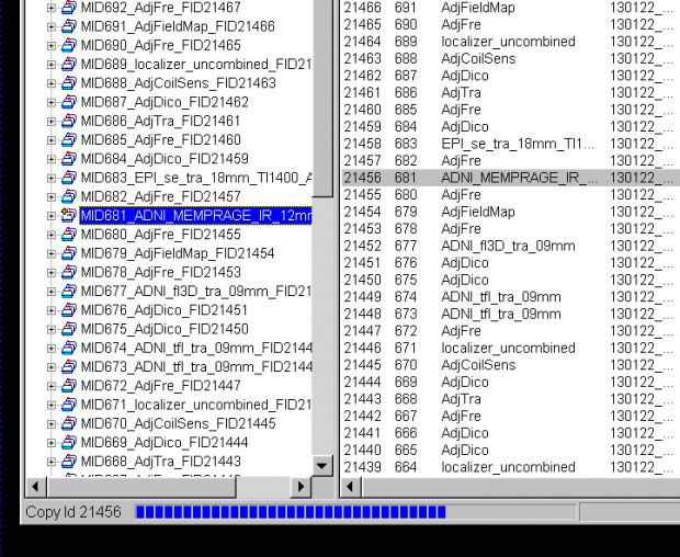
At times, it may be useful to save the raw MR data that is acquired in the receiver coils, prior to image reconstruction in the MR Image Reconstructor (MRIR). This can be used by Siemens or Ross in diagnosing problems in novel sequences or with image reconstruction. Its unfeasible to always save this data as the files can be very large – a 8 min BOLD scan with the 32-channel coil might be ~ 20 GB in size. However, Ross may ask you to save this data if you’re having problems with your images. Here’s how to do it.
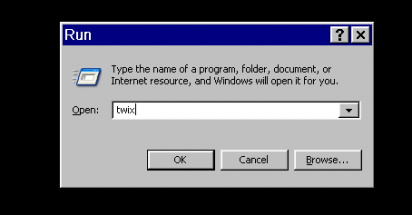
- Open the Windows XP Run window from the bottom menu, using Ctl-Esc. When the Run window appears, enter
twixand hit the OK button.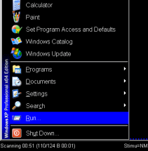
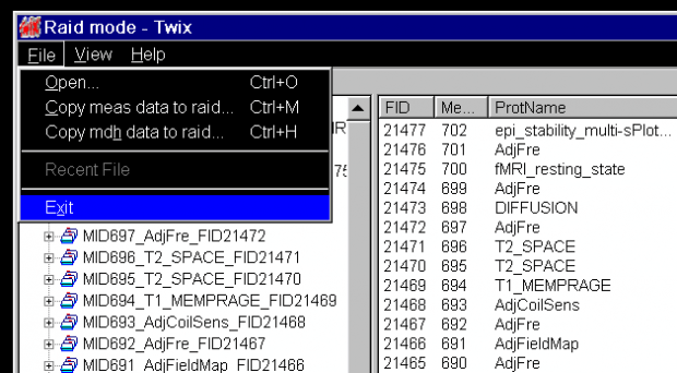
- The application Twix opens over the Syngo display. This lists all the scans for which data is still on the MRIR, in reverse chronological order. The listing is done twice – on the left side, where just the scan name and measurement ID is given, and on the right, where the file size, date and time, etc, is also listed. Scroll down the left side to find the scan you want to save the raw data for (
ADNI_MEMPRAGEin this example) and click on it once, so it is highlighted. The corresponding row in the right display will also be highlighted (allowing you to check it’s the right scan).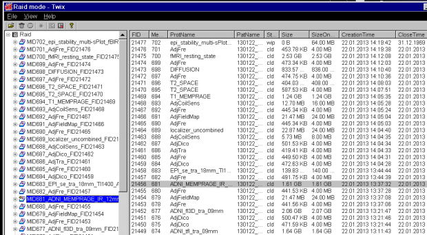
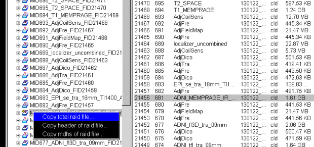
- Now, with the mouse over the file name in the left column, right click to bring up the pop-up menu, and then choose the first option Copy total Raid file:
- A Save-file pop-up window will now appear. You can choose the default name and location to save the file on the scanner host computer, or enter your own preferred location, eg:
T:\User: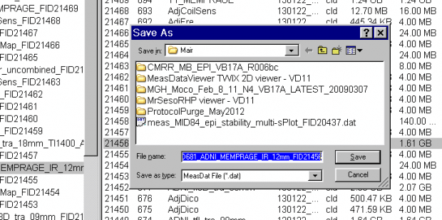
- Click the Save button. A status bar showing the progress of the file being saved is seen at the bottom of the TWIX window.
- Once the status bar in the Twix window showed the saving operation had completed (the status bar then disappears) now you can exit TWIX. Return to normal scanner operation. Send Ross (rmair@fas.harvard.edu) an email saying you saved a raw data file, including the time and the 4-digit ID.
How is the performance of the scanner monitored?
The performance of the Prisma system is monitored via a series of daily and weekly scan protocols. Daily QA scans on a large water phantom ensure:
- High temporal SNR for functional MRI
- Consistent single image SNR and minimal/consistent image ghost intensity in EPI scans for functional and diffusion weighted MRI
- Lack of RF interference from other equipment and lack of gradient spiking that could cause image artifacts.
Weekly QA scans using a structured phantom are used to assess gradient non-linearity and image distortion.
In addition, we have begun using the fBIRN agar phantom on a 1-2 weekly basis to also document EPI time series stability, drift and temporal SNR in a manner consistent with other fBIRN sites.
SMS/Multiband
In what order does the scanner acquire EPI slices for SMS/multiband scans?
In simultaneous multi-slice (SMS)/multiband acqusitions, multiple slices are acquired at the same time. If you’re doing any form of slice-time correction with your data, you need to be aware of this, and know how find the slice time information in each scan, as traditional slice time correction algorithms wont work.
If you’re using dcm2niix to convert your DICOMs, use the -b flag to generate the BIDS .json header-information file. This file will contain the slice-time information for each scan. Alternatively, the slice-time information is accurately detailed in the DICOM header of your SMS_BOLD images. The information is in DICOM field 0019,1029. This is part of the Siemens dedicated section of the header – some command line tools that are part of, eg. Freesurfer or AFNI may not show the information. But DICOM viewer programs like Horos version(Mac) or Syngo FastView (Windows) will show this information in the tabulated view of the DICOM header. Unfortunately, DicomBrowser on FASSE doesn’t show the information, so you will need to transfer one of the DICOMs from a run to your local machine by following these instructions.
While you should always check the DICOM header for the accurate slice-time information for your protocol, we have put the slice-time information for commonly used protocols in the FASSE environment here:/ncf/mri/01/users/shared/slice_times_for_SMS/VE11C_2017_2019
(See here for how to download these files, or here for how to just view them.)
How do I convert my SMS images correctly?
The only reason there is any difference in converting SMS-BOLD images is that the numbers coming out of the SMS-BOLD scans are larger, which can be a problem for some older conversion programs if they aren’t reading the bit format correctly.
The voxel intensity range used to be (and for Siemens sequences, still is) 0-4095. For the SMS-BOLD sequence from Minnesota, the intensity range is 0-65535. This was done because as high-array head coils (32ch, 64ch) have come to predominate, the range of intensities across the head has become much larger than it used to be in the days of the 12ch (or 4ch, or 1ch!!) coils. To avoid getting trivially low numbers in the middle of the brain, everything has been scaled up.
Some DICOM conversions would fail for voxel intensities above 32768 – anything above that gets converted a large negative number, which can look like black voxels where there should be bright white ones. This would usually happen at the top of the head where the numbers are largest. If you have image series where no voxels have values above 32768, then the old routines will still work.
There are various solutions based on your analysis program.
SPM: avoids converting, so you don’t have to worry – unless you like to take the output from SPM and input it into another program, then you should verify the conversion happens correctly.
mri_convert/Freesurfer: This is part of freesurfer, and also used by fc-fast. Freesurfer versions 6.0 and higher can handle this data without issue. If you’re still using an older Freesurfer version please source the module below. The mri_convert module MUST be sourced after you source your freesurfer version. For instance, if you want to run fc-fast, you should source the following, with the last line being the critical module for the fixed mri_convert.module load freesurfer/5.3.0-ncf
module load mri_convert/2015_11_09-ncf
AFNI: in to3d you need to include the –ushort2float flag. This is only available in the newer versions of AFNI (available via list_loaders or through modules). So make sure you are loading a more recent version than the default.
dcm2niix: Handles data in this format by default. (Do not use older dcm2nii versions)
How do I acknowledge the SMS-BOLD sequences and the Prisma scanner?
See the Acknowledgements and Citations page.
What is the SBRef image? Or why does each scan show up as two in CBSCentral?
You should notice a single time-point image with “_SBRef” appended to the series name, for each one of your SMS-BOLD scans:
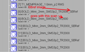
This “Single-Band Reference” image is what the scanner is acquiring during the 10-20 seconds of reference scans before the first trigger is sent, and your first real time-points are acquired. This image matches your real brain-volumes, but is just acquired without slice acceleration. The scanner is acquiring it anyway, so why not have it stored with your data?
The WashU/UMn HCP consortium recommend using this SBRef image as the starting point for motion correction, and for alignment of your BOLD images to anatomical images. Especially if you’re using a short TR, the SBRef image will have superior SNR and contrast to your BOLD scans, which is why this method is suggested.
See: Glasser et al, The minimal preprocessing pipelines for the Human Connectome Project, NeuroImage 80 105–124 (2013).
In what order does the scanner acquire EPI slices in non-SMS scans?
If you have multi band/SMS data, please see above. The following information only refers to traditional non-SMS scans, and is included here for historical reference only.
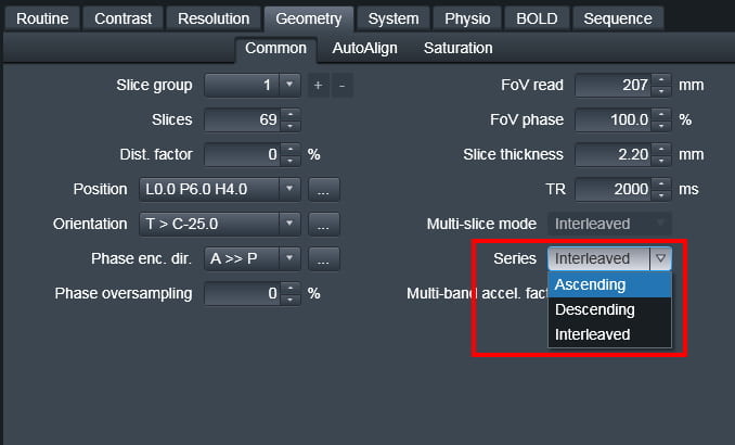
There are three options for slice ordering for EPI. To understand the ordering you first need to know the Siemens reference frame for the slice axis: the negative direction is (Right, Anterior, Foot) and the positive direction is (Left, Posterior, Head). The modes are then:
Ascending – In this mode, slices are acquired from the negative direction to the positive direction (foot to head for axial slices)
Descending – In this mode, slices are acquired from the positive direction to the negative direction (head to foot for axial slices)
Interleaved – In this mode, the order of acquisition depends on the number of slices acquired. If there is an odd number of slices, say 27, the slices will be collected as:
1 3 5 7 9 11 13 15 17 19 21 23 25 27 2 4 6 8 10 12 14 16 18 20 22 24 26.
If there is an even number of slices (say 28) the slices will be collected as:
2 4 6 8 10 12 14 16 18 20 22 24 26 28 1 3 5 7 9 11 13 15 17 19 21 23 25 27.
Interleaved always goes foot to head, i.e. negative to positive direction.
The slice order is set from the “Series” pull-down menu on the Geometry tab. Do not confuse this with the “Multi-slice-mode” option on the same tab, which would seem to be the more logical name for this parameter – but isn’t.
The time that each slice is acquired within the TR can be found in the DICOM header. Contact Ross at rmair@fas.harvard.edu if you need information on this.
How do I use the slice order information in my analysis
Why do we use interleaved slices?
For EPI-BOLD scans, the majority of users use interleaved slices; for instance, all odd slices followed by all even slices: 1,3,5,7,…2,4,6… By interleaving, a time of TR/2 is left between the excitation of any one slice and either of its next-nearest neighbors, thereby minimizing crosstalk (partial saturation) between them and maximizing SNR. For SMS-BOLD scans, interleaving is always used by default, and attention is paid in the slice ordering to prevent adjacent slices being excited in a time less than TR/2.
Historically, interleaving was used to overcome the imperfect RF profile of the excitation RF pulse. In an ideal world the frequency profile – and hence the spatial profile of the slice selection pulse – would be a perfect square. In reality, however, excitation RF profiles tend to be more trapezoid-like. The first consequence of non-square slice profiles is one of nomenclature. When we talk about slice thickness and slice-to-slice distances we need to define the point on the profile we’re using as our reference. The standard convention is to take the half-height width as the slice width, and define inter-slice distances accordingly. This is not a universal rule, however, and empirical testing by those at UC Berkeley suggests that Siemens uses something like 5% or 1% above baseline to define its slice thickness. (In other words, when you ask for a 3 mm slice the base of the trapezoid would be 3 mm but the half-height might be only 2.95 mm.) Now let’s look at the inter-slice overlap issue from a practical standpoint, and address the issue of interleaving. The Berkeley study revealed that with sequential slices, the slice SNR remained at its maximum (100%) level when using gaps of 5-20%. Only when the gap was reduced to a nominal 0% gap was there a very slight decrease of image SNR, to 99%. (This is how we estimate the Siemens convention of using the base of the trapezoid to define slice width.)
These results have two consequences. Firstly, it means that you can use gaps of 5-20% without getting appreciable saturation effects, and even no slice gap has minimal effects. Secondly, the implication is that interleaving isn’t necessary to mitigate slice crosstalk; the slice profile takes care of most of it.
Now that we have seen there is no strict reason, other than historical precedent, to use interleaving, what are the differences between interleaved and sequential slicing? Does one provide a definite advantage over the other? In the absence of head motion the answer is ambiguous: there is almost no difference in performance. But whenever the subject moves his head in the slice dimension (through slice movement) the consequences for interleaved slices can be more severe than for sequential slices. In the case of sequential slices, the movement would cause some new anatomical regions to be included at one end of the slice stack, while some other anatomical regions disappear from the other end; i.e. the brain moves through the slices. The same motion would cause a slice-to-slice signal intensity variation when using interleaving, but only for the duration of the movement. That is because as the movement occurs we are going “up and back through” with the slices, rather than slicing in a single direction, as with sequential slices. In effect, it is as if we have changed the effective TR for the slices.
So what is the best approach? The most robust approach seems to be using sequential slices acquired head-to-foot, or in descending order. Sequential slicing will avoid the striping that might happen because of certain types of head motion, while going “top to bottom” with the slices will minimize interference from the inflowing blood (ASL-like) enhancement of functional contrast. However, the requirements of SMS-BOLD scans to keep adjacent slices from being excited close in time have made the interleaved approach the default method for such scans.