Imaging Data Analysis

See here for what software is available and how to access it.

(jump link)

You can change your SPM version similar to any other brain analysis software using the tools described above. We recommend using module load spm/12.7487-fasrc01.  However, you also need to add the SPM version to your MATLAB path.  You can do this by using one of the variables set in the default unix environment, $_HVD_SPM_DIR.  To check what that variable is set to, type:

echo $_HVD_SPM_DIR

Remember, if you want to use a different version of SPM on future logins and in different terminals, you must add it to your .bashrc file. Once you have the SPM you want you can add this variable to your ~/matlab/startup.m file (See here for editing files).

addpath(getenv('_HVD_SPM_DIR'));

This will prepend SPM and its subdirectories to your MATLAB path, which means it will supersede any version you had previously set in your path.  You should be aware that if you make changes to your path in MATLAB and then save it, this version of SPM will become part of your ‘permanent’ path, as it was added on the fly at startup, but then you just saved the whole current thing.  This can become a problem if you are switching back and forth between versions.  This is also true of Freesurfer, which likes to add things to your MATLAB path, so make sure to check this occasionally and make sure multiple things aren’t added (via Home -> Set Path on the menu bar in MATLAB).

(jump link)

A collaboration with IQSS (Alex Storer), a previous graduate student, Caitlin Carey, and our local Tim O’Keefe have resulted in a set of python scripts to help you with your SPM analysis. They are designed to take a batch script you create for a single subject, and apply it to a bunch of subjects. They start by downloading your data from CBSCentral. So even if you don’t want to use them for analysis, you might want to use them for grabbing your data and converting to SPM niftis. The instructions for using them are located on the NCF GIT site. The scripts do not have to be downloaded, but you do have to load the module for them. In your script, or in your terminal window, you will need to have the following commands before you can use or even see them.

module load ncf
module load spmtools-centos7/1.0-ncf

You should load what ever the latest tag is, as master is the code that gets updated.

The instructions for use are located here: https://ncfcode.rc.fas.harvard.edu/mcmains/spmtools-centos7/blob/master/README.md

Essentially, they replace the path information in your batch script with that of the new subject. You can easily check the new batch created for correctness, and make an additional specialized updates you want. They have been tested with basic preprocessing (including SPM12 where you can include slice timing information for SMS/multiband scans), through your first level analysis.

(jump link)

Using SPM:

It is easy to add the fieldmap into your preprocessing batch, via SPM -> Tools -> FieldMap -> Presubtracted Phase and Magnitude Data.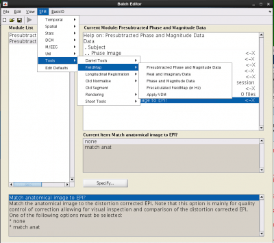

Phase Image: load your phase image

Magnitude Image: load the mag image with the shortest echo time (usually the first)

Fieldmap defaults: Select Defaults values. This will expose several all things to enter:

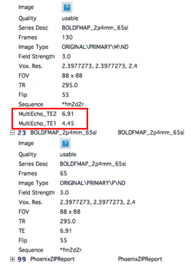
• Echo times [short TE long TE]: Enter the two echo times from your fieldmap. These can be found on CBSCentral or in your protocol.
  
• Mask brain: Mask brain
• Blip direction: -1 (but really this partly depends on how you convert your dicoms, so for your first subject, you should try it both ways and see which way is better. See the end of the instructions for what is ‘Better’.
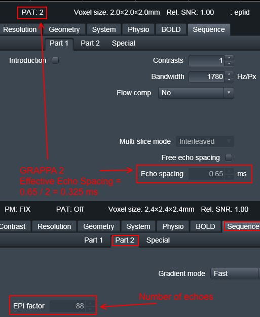
• Total EPI readout time: This will be the EPI factor*echo time for the BOLD you want to unwarp. These two values can be found in the protocol pdf print out (email Ross if you don’t have it (rmair@fas.harvard.edu), or on the scanner. If you use GRAPPA (iPAT) you need to divide the echo spacing by the pat factor (highlighted at the top of the pic below in red)
  
• DPI-based fieldmap: non-EPI
• Jacobian modulation: Do not use
• Everything else you can leave at the default values

EPI Sessions: Create a session for each one of the runs you want to unwrap, then select the first image of each run.

Match VDM to EPI?: select match VDM

Write unwrapped EPI?: You do not need to put this in, but if you do, you will get more info in the window after it runs that will allow you to check the quality.

Select anatomical image for comparison: Select your structural image. This is also just for quality control.

Match anatomical image to EPI?: Select match anat, though again just for QC.

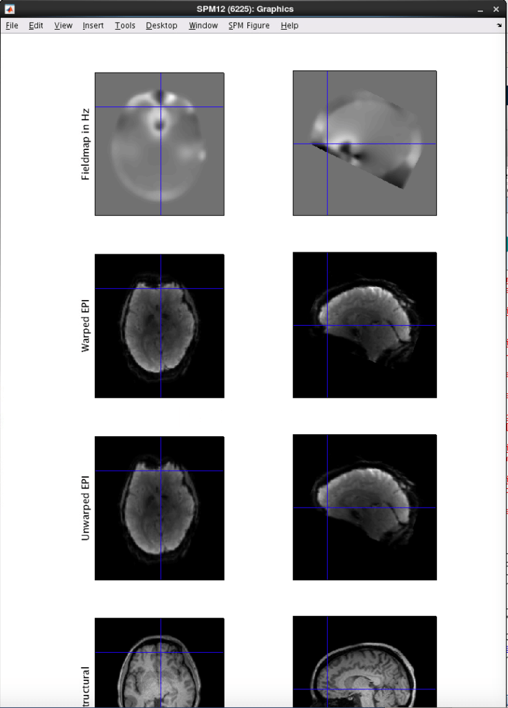
See the bottom of this post for an example of the output. You should click around and make sure things look good. You want the BOLDs to extend further anterior in the area of dropout by the eyes, as you can see below, with the unwarped EPI (with the fieldmap applied), extends further anterior than the warped EPI.

Using FSL:

There is a very thorough tutorial located here: https://fsl.fmrib.ox.ac.uk/fslcourse/lectures/practicals/registration/index.html

FSL Prepare Fieldmap: You will need to know the difference in echo times for your fieldmap. This can be seen at the scanner on the Routine tab, or from CBSCentral, by looking at the scanning specs for the first scan of the fieldmap (see above for an example). You just subtract the two numbers.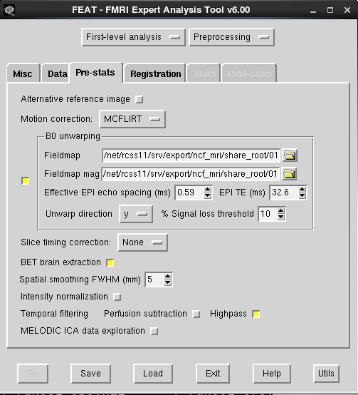

Feat GUI:

• Effective EPI echo spacing: This is referring to the BOLD scan you want to unwarp, and can be found on the scanner or the protocol pdf print out, see the image above. If you use GRAPPA, this must be divided by the iPAT factor (highlighted in the red box at the top of the picture above in the SPM directions for the scanner protocol tabs this can be found on. If your BOLD protocol uses GRAPPA, you need to divide the echo spacing by the iPAT factor.
• EPI TE: this is the TE of the BOLD you want to unwarp (not the fieldmap), this can be found in CBSCentral.
• Unwarp direction: This can be affected by how you convert your dicoms, so the safest way to figure this out is to try it both ways for your first dataset. You want the BOLDs to extend further anterior in the area of dropout by the eyes. If you can not tell, feel free to email Ross (rmair@fas.harvard.edu) and ask him to take a look at your data. For an example, the unwarped EPI (with the field map applied), extends further anterior.

(jump link)

To use your spin echo fieldmap data, you will first have to transform it into a more traditional fieldmap. This can be done using FSL’s program called Topup. this was originally made for working with DTI data, but also works for BOLD. The instructions are the same for using this in SPM or FSL until the last steps, so we will start with the common directions first.

First, make sure you have FSL version 5.0.9 or later. See here for how to select your version of FSL.

Then, generally follow the instructions from FSL, with some helpful notes below: https://fsl.fmrib.ox.ac.uk/fslcourse/lectures/practicals/fdt1/index.html#topup.

You want to start with the section labeled Running topup.

The two files you want to merge are your two fieldmaps, which are the same thing, but collected in opposing encoding directions (Anterior to Posterior and Posterior to Anterior).

Topup command: you want to make sure to specify the iout and fout flags. The config file is the default file that fsl provides. This should work in most cases.

topup --imain=ap_pa_merge --datain=acqparams.txt --config=b02b0.cnf --out=topup_results --fout=fieldmap --iout=unwarped_images

Make a single mag image:

fslmaths unwrapped_images -Tmean myfieldmap_mag

For FSL, you will need to skull strip this:

bet myfieldmap_mag myfieldmap_mag_brain

This is where the two packages diverge.

SPM:

In your spm batch, select SPM -> Tools -> FieldMap -> Precalculated FieldMap (in Hz).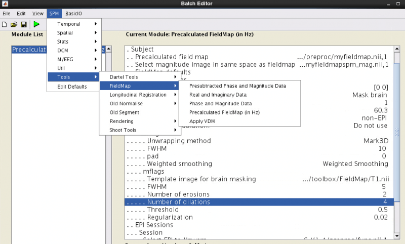

Precalculated fieldmap: load the fieldmap you created, fieldmap.nii FSL likes to make gzipped files, so you will probably have to unzip this first (gunzip fieldmap.nii.gz)

Selected magnitude image in same space as fieldmap: myfieldmap_mag (again you might have to unzip)

Fieldmap defaults: select Defaults values, which reveals more variables

• Echo times: [0 0] (because they aren’t used)
• Mask brain: Mask brain
• Blip direction: This could be 1 or -1, it partly depends on how you convert your dicoms, so try it both ways and compare, you want the brain in the orbital frontal areas to extend further forward. If you can’t tell, ask Ross (rmair@fas.harvard.edu) for help.
• Total EPI readout time: This will be the EPI factor*echo time of your BOLDs again. These two values can be found in the protocol pdf print out (email Ross if you don’t have it (rmair@fas.harvard.edu), or on the scanner. If you use GRAPPA (iPAT) you need to divide the echo spacing by the pat factor (highlighted at the top of the pic below in red)
  
• EPI-based fieldmap?: non-EPI
• Jacobian modulation: Do not use

The rest can be left with the default values.

EPI Sessions: Create a session for each one of the runs you want to unwrap, then select the first image of each run.

Match VDM to EPI?: select match VDM

Write unwrapped EPI?: You do not need to put this in, but if you do, you will get more info in the window after it runs that will allow you to check the quality.

Select anatomical image for comparison: Select your structural image. This is also just for quality control.

Match anatomical image to EPI?: Select match anat, though again just for QC.

After you run it, check the output that is created. You want the data to look ‘better’ after unwarping. If you can not tell, feel free to email Ross (rmair@fas.harvard.edu) and ask him to take a look at your data. For an example, the unwarped EPI (with the field map applied), extends further anterior.

FSL:

For FSL, the fieldmap must be converted to radians:

fslmaths fieldmap.nii.gz -mul 6.28 fieldmap_rads

Then in the FEAT fieldmap gui, you want to use fieldmap_rads as the fieldmap, and the brain extracted unwarped image as the mag (myfieldmap_mag_brain).

Effective EPI echo spacing: This is referring to the BOLD scan you want to unwarp, and can be found on the scanner or the protocol pdf print out, see the image above. If you use GRAPPA, this must be divided by the iPAT factor (highlighted in the red box at the top of the picture above from the scanner.

EPI TE: this is the TE of the bold you want to unwarp (not the fieldmap), this can be found in CBSCentral or at the scanner.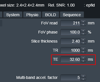

Unwarp direction: This can be affected by how you convert your dicoms, so the safest way to figure this out is to try it both ways for your first dataset. You want the BOLDs to extend further anterior in the area of dropout by the eyes. If you can not tell, feel free to email Ross (rmair@fas.harvard.edu) and ask him to take a look at your data. For an example, the unwarped EPI (with the field map applied), extends further anterior.

(jump link)

First, see here for how to determine the slice order of your scan for SMS/multiband sequences and non-SMS sequences.

Because the order of slices is dependent upon the scanner type, slice acquisition type, and number of slices, most MRI analysis packages have a place to put this information in. It is most commonly used during slice time correction, which needs to know the order of slices to correct for the difference in acquisition time for each slice. 

SPM

In the slice timing module, you need to set the slice order (see here for more details, which differs for odd/even interleaved slices, and for every protocol if using SMS/multiband ), and you must set the reference slice, or the slice to be corrected to. [See below for information and issues on reference slice selection] 
For SMS scans, you must use SPM12 or newer, which allows you to enter a time that each slice was collected. In general, people have then been choosing the reference slice to be the first one, or 0 for time 0.

AFNI

You must set the order of slices regardless of if you plan to do slice time correction or not, within to3d: For interleaved odd: alt+z, interleaved even: alt+z2. Then, if you perform slice time correction, you can set the reference slice within 3dTshift. 
For SMS scans, you must read in a text file with the timing for each slice. This should be provided in to3d and 3dTshift, where it might be safest to choose the first slice as the reference.

PROCFAST

A homegrown script from the Buckner lab for preprocessing. This script has hardcoded information about slice order and the reference slice. It assumes the interleaved odd slice order (1,3,5,2,4) for all data, and chooses the middle slice as the reference (using the odd slice order). If you have data with an even number of slices you can either 1) edit the information within fsl_preprocess, the script that does the slice time correction. This can be done by copying fsl_preprocess to your local directory, editing it, and adding it to your path so that it is used. You need to edit line 210 for the slice order (sliceOrder) and 231 for the reference slice (middleSlice). Alternatively, if you just want to change the slice order, you can do this by setting the variable sliceOrder. In bash, type: 
export sliceOrder=”2:2:<# of slices> 1:2:<#of slices>” 
where <# of slices> is replaced by the number of slices you have. You can verify that your changes worked by looking at the output of the script. Shortly after it says ‘Performing slice time correction’, the script launches MATLAB. Right at the beginning of the MATLAB call it gives the slice time correction command, you want to make sure the numbers shown below are correct: 

Warning: Unable to open display iconic, MATLAB is starting without a display. 
You will not be able to display graphics on the screen. 

< M A T L A B > 
Copyright 1984-2007 The MathWorks, Inc. 
Version 7.4.0.287 (R2007a) 
January 29, 2007 

To get started, type one of these: helpwin, helpdesk, or demo. 
For product information, visit www.mathworks.com. 
>> spm_slice_timing_noui(P,[2:2:12 1:2:12],2 4 6 8 10 12 1 3 5 7 9 11,[3/12 (3 - 3/12) / (12 - 1)]) >> 
SPM2: spm_slice_timing_noui (v2.20) 16:15:18 - 11/08/2011 ======================================================================== 
 

As procfast uses an old version of SPM for slice-time correction which cannot handle SMS acquisitions; if you have acquired SMS data you can’t use the default version of procfast. However, you can bypass slice time correction completely in this case. Send an email to our neuroinformatics group (info@neuroinfo.org) for details on a work-around that skips the slice time correction step.

Note on Reference Slice:

Often, people use the middle slice as the reference slice with the reasoning that the most any slice will be corrected by is ½ a TR. However, this has implications for the timing of your stimuli, as you just essentially shifted your 0 point by half a TR. To correct for this, your stimulus onset times need to be shifted back by half a TR (i.e. times = times-1/2TR). Alternatively, for simplicity, some people correct to the first slice, this eliminates the need for any correction of your stimulus onset times. There is some controversy about whether SPM can correctly read the slice order/reference slice information when performing a FIR analysis to extract time course information (reported 11/2011). This seems particularly an issue when taking the output from procfast. Therefore, it is recommended to use the first slice as the reference in this case.