Need help with something QC-related? Here’s who to ask for help!
| Issues with: | Contact: |
|---|---|
| General help CBSCentral Excessive motion during scan Qualitative QC walkthrough | Jenn Segawa (jsegawa@g.harvard.edu) |
Individual scan protocols RF/Spiking or ghosting in scans | Ross Mair (rmair@fas.harvard.edu) |
Slides from QC workshop
Click here for slides from the QC workshop presented by Natasha Hansen (natasha.s.hansen@gmail.com). The workshop slides give a comprehensive overview of quality control for MRI data including why QC is important, the kinds of QC: quantitative vs qualitative, quantitative QC measures in XNAT, and qualitative QC with artifact examples and unusual cases. Don’t miss out on the accompanying manual on qualitative QC below!
Quantitative QC: Automatic BOLD QC via CBSCentral
How do I run the extended bold QC on CBSCentral?
If you have your functional data in CBSCentral labeled as type BOLD, then the extended bold QC pipeline will automatically be run on your data, shortly after it is archived. The type of your scan is set when you manually archive your data. See the image below for an example.
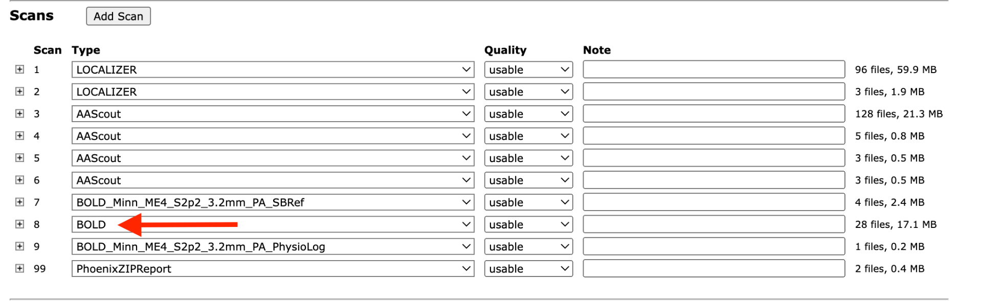
If you previously used the scan type to specify study specific information, like bold_run1, you will need to move that information to the notes field.
What does the automatic BOLD QC do?
The pipeline:
- Converts the dicoms to nifti format,
- Creates mean, standard deviation, and SNR maps,
- Calculates slope and mean slice intensity changes and then
- Performs motion correction (with MCFLIRT from FSL) to get measures of movement.
What files are produced?
The results will be uploaded to CBSCentral separately for each subject and each run. You can get to the BOLD QC data by: a) clicking the scan name under the Assessments heading at the bottom of the session info page or b) clicking the View links in the QC column under the Scans heading.
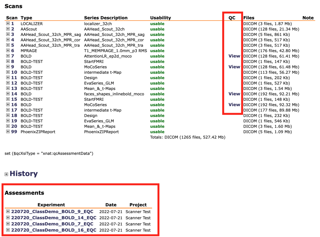
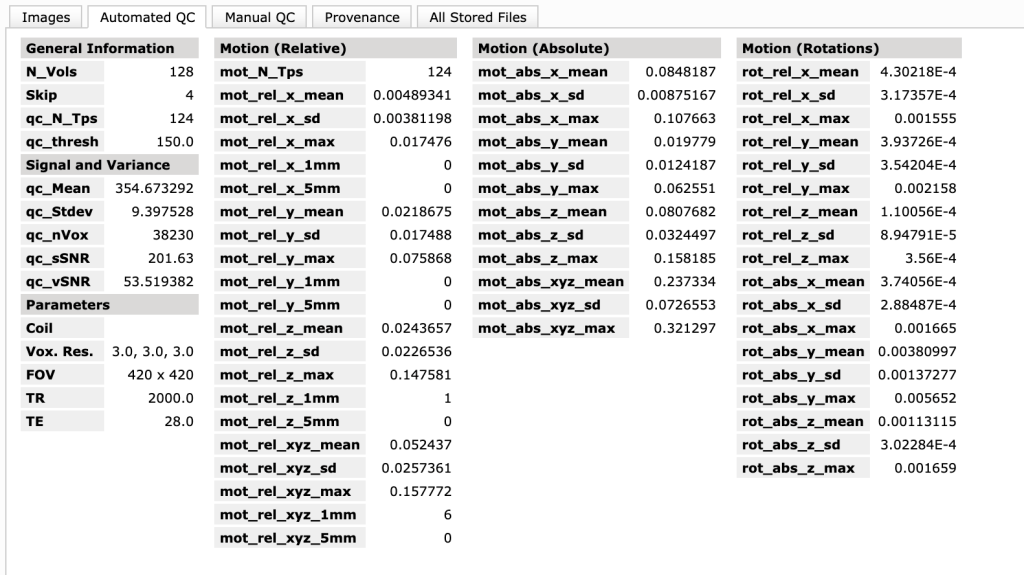
This will take you to the scan’s QC page, which looks like this:
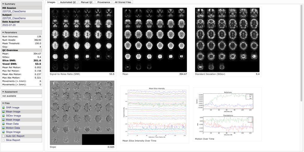
Which QC measures are important?
The parameter’s box on the left side has a lot of useful statistics. This contains several measures the Buckner lab has found to be useful in determining whether a dataset is usable or not. These have been developed by looking at many datasets over the years and are rough guidelines that work specifically for Siemens 3T 12 channel data from adults. To get a description of what a parameter is, hold the mouse over it.
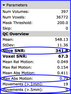
Three measures to start with are:
- Slice SNR: Measures the timecourse SNR (mean/stdev) averaged across each slice, and then averages all the slices together. This serves as a general ‘goodness’ measure. If it is greater than 150 , then the data is good, while less than 99 is bad (for Siemens 3T 12ch adult data). This number can be low for several reasons, including subject motion and scanner artifacts. A low value should be a red flag to look more closely at the data.
- Max Abs Motion (maximum absolute motion) is also useful for determining usability of data. Values less than 1.49 are good, while greater than 2mm is bad.
- Movements (>.5mm) (Number of movements greater than 0.5mm) should be less than 5 for good data, greater than 5 is bad. This is calculated as the root mean square of movement in 3D space.
There are many other variables listed that you might find useful, but for which we haven’t developed hard guidelines for. For instance, voxel SNR (timecourse SNR calculated for each individual voxel) is more dominated by scanner noise than slice SNR and might be useful. So might be max or mean relative motion, which is movement relative to the previous volume as opposed to the first volume.
What graphs and pictures are displayed (under the Images tab)?
- Top Left: Voxel SNR map
- Formed by dividing the mean map (middle map) by the standard deviation (right map).
- Generally, it will take some practice in looking at these maps to tell what is ‘normal’, and this varies by coil. For the 12ch, you generally want the mean and SNR map to be uniform. For the 32ch, these are generally brighter at the edges of the brain.
- Middle Left: Slope Map
- Calculates changes over time, and therefore can be useful in highlighting movement. Areas of white or black have large movement.
- Middle Center: Mean slice intensity over time
- You want these lines to be fairly smooth
- Middle Right: Motion parameters
- From MCFLIRT (affine registration, FSL)
- You also want relatively small changes.
- Check the axis scale closely to interpret the magnitude of the movements.
- Bottom: Mask
- You want this to be generally uniform and covering the whole brain. If there are areas of drop out, this might suggest regions of low signal.
What is the Automated QC tab?
This tab shows a few more measurements than the main summary page, in addition to everything on the summary page.
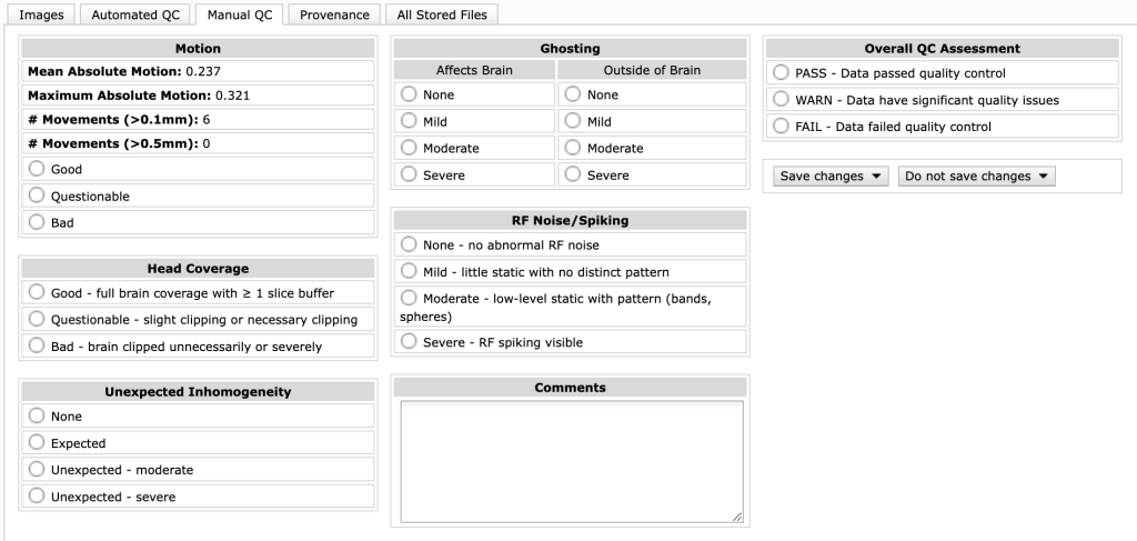
What is the Manual QC tab?
In this tab, you can record overall ratings of the data, which can later be read by other users or can be used to filter ‘usable’ data in the database. There are several criteria by which data can be classified. These include motion, head coverage, signal homogeneity, ghosting, and RF noise/spiking. Motion can be assessed with the quantitative values that come out of the CBSCentral automated extended BOLD QC, while the rest need to be assessed via qualitative inspection of your data. Then, there is a final overall QC assessment rating that can be set.
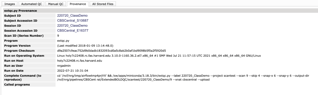
What is the Provenance tab?
This contains the scripts that were run in case you want to recreate something on your own.
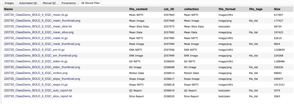
What is the Stored Files tab?
This is where the files created are listed. You can click on any of these to download the files. Currently, these download with extra information on the beginning and end of the file name. We are working to correct this. The last two are the report files. The auto_report.txt file contains the statistics from the extended BOLD QC that can be used to qualify data. The slice_report.txt contains mostly the slice-based SNR measurements.
How can I create my own standards for what is usable data?
This might be necessary if you are scanning a non-typical protocol, such as on children, patient populations, or with a different coil.
The easiest way to create new standards is to look at the values across all of your subjects in an experiment. You can calculate the average value for the important parameters discussed above and then look for outliers. You can do this by recording key parameters manually or by clicking on the report files from the ‘all files’ tab or on the left hand side of the main page. Currently, these download with extra information on the beginning and end of the file name. See below for how to interpret the files.
How do I interpret the report files?
The auto QC report contains the parameters in the parameters box on the left, in rather cryptic names:
- qc_sSNR = slice SNR
- qc_vSNR= voxel SNR
- mot_rel_xyz_mean = Mean Relative Motion
- mot_rel_xyz_max = Max Relative Motion
- mot_abs_xyz_mean = Mean Absolute Motion
- mot_abs_xyz_max = Max Absolute Motion
- mot_rel_xyz_1mm = Number of movements > 0.1mm
- mot_rel_xyz_5mm = Number of movements > 0.5mm
The slice report contains the slice SNR, slice mean, slice stdev, slice mean min and max across all timepoints, and the number of timepoints considered outliers. These are reported separately for each slice, and then averaged together in the end. This is where the slice SNR displayed in the parameters box comes from.
Qualitative QC: Looking at your data
Click here for a qualitative QC manual (pdf) created by Natasha Hansen et al. (natasha.s.hansen@gmail.com). This manual is a great starting place for learning about QC. It provides mild, moderate, and sever examples of all of the artifacts you want to look for in your data.
MRI Qualitative Quality Control Manual, (2013). Natasha Hansen, Garth Coombs, Thilo Deckersbach, and Randy Buckner
In addition, there is a useful video on how to use FSL to perform qualitative QC. Note that the video is older and uses deprecated software (FSLView). Contact Jenn Segawa (jsegawa@g.harvard.edu) for access.
How do I perform qualitative QC on my structural data?
Qualitative QC involves looking at your data. We recommend doing this via FSL. This does not mean you need to analyze your data in FSL, but the FSLeyes just has a nice interface to visualize the nifti files. After you finish the qualitative QC you can enter your findings into CBSCentral using the manual tab. For a better description of the various artifacts, see the QC manual (pdf).
- Load your structural scan. If you are using FSL (if do this on a Remote Desktop, don’t forget to run
module load ncf fslfirst), type:fsleyes structural_name & - Scroll through all the slices in each view of the brain.
- Verify that that all of the brain is there (not clipped)
- Verify that if any part of the anatomy fell outside of the field of view and is wrapping around, that it doesn’t overlap with the brain.
- Look for artifacts in the ‘ringing’, ‘striping’, and ‘blurring’ category. These artifacts can sometimes be easier to see if you use Single View (Tools > Single) to enlarge the view of the axial plane.
- Look for radio frequency (RF) noise, which resembles TV static over the scan image, and spiking, which looks like rigid stripes over the brain and/or background.
- Look for susceptibility artifacts (a black area of signal loss surrounded by bright and dark ripples – such as in the mouth when participants have a permanent retainer).
- Turn on Lightbox View (Tools > Lightbox) and scroll down to slices that show the full walnut shape of the brain. Decrease the contrast by lowering the max brightness value while leaving the minimum brightness as the default value (0). Lower the max brightness to 1/3 the default value. Scroll through all the slices:
- Look for ghosting (a fainter displaced copy of the head, brain, or eyes).
- Pay attention to where the ghost image might overlap with the brain.
- Look for RF noise. With this contrast, a little RF noise (TV static) is normal, but you should check if there is more than usual. You should not see rigid stripes (spiking).
- Reset the brightness values to default. Then increase the contrast by raising the minimum brightness value while leaving the maximum brightness value at the default. Raise the minimum brightness to 1/3, then 1/2, then 2/3 of the maximum, each time scrolling through all the slices in each view of the brain.
- Look for the homogeneity of the signal intensity. You will get to know what looks normal for your scanner and coil, but in general the outer rim of the brain is brighter than the interior. The signal homogeneity pattern should be symmetrical, particularly left to right. In general, it should also be symmetrical front to back, but if you use the 32 channel coil this will depend on how the subject’s head was padded.
How do I perform qualitative QC on my functional data?
Qualitative QC involves looking at your data. We recommend doing this via FSL. This does not mean you need to analyze your data in FSL, but the FSLeyes just has a nice interface to visualize the nifti files. After you finish the qualitative QC you can enter your findings into CBSCentral using the manual tab. For a better description of the various artifacts, see the QC manual (pdf).
- Load your functional data. You will have to perform QC for each BOLD run. If you are using FSL (if do this on a Remote Desktop, don’t forget to run
module load ncf fslfirst), type:fsleyes functional_name & - Check for head coverage, make sure all of the brain target area (the part you care about for your study) is covered and not clipped by the edge of the field of view.
- Remember to scroll through all the slices in the coronal plane to check if the bottom tips of the temporal lobes are cut off.
- Turn on Movie mode. This will automatically cycle you through the timepoints (volumes), so you will be more likely to spot issues that are timepoint-specific as you scroll through the slices. Continue to scroll through the slices, making sure that movie mode plays through a full cycle of volumes and starts over at zero (0) several times.
- Look for motion slice artifact (sudden horizontal light and dark stripes through the brain that may only be there for particular timepoint(s).
- Look for RF noise (like TV static) and spiking (sudden extreme static and/or stripes through the brain). Mild-moderate degrees of RF noise can be more easily seen when you decrease the contrast (see step 7 below).
- Turn on Lightbox View (Tools > Lightbox) and increase the view size to 200%.
- Scroll though all the slices in each view of the brain.
- Decrease the contrast by lowering the maximum brightness value to 1/3 the default while leaving the minimum value at the default (0). Scroll through the slices in each plane:
- Check for ghosting (a fainter displaced copy of the brain). There will always be some amount of ghosting, but check how visible it is and is if it overlaps the original brain image.
- Look for RF noise and spiking again.
- While leaving on Lightbox and Movie mode, reset the contrast to its default values. Then increase the contrast by raising the minimum brightness value while leaving the maximum at the default. Raise the minimum brightness to 1/3, then 1/2, then 2/3 of the maximum, each time scrolling through all the slices in each plane.
- Look for the homogeneity of the signal intensity. You will get to know what looks normal for your scanner and coil, but in general the outer rim of the grain is brighter than the interior. The signal homogeneity pattern should be symmetrical left to right. In general, it should also be symmetrical front to back, but if you use the 32 channel coil this will depend on how the subject’s head was padded.
Preventative QC: At the scanner
How do I monitor movement in real-time using FIRMM?
FIRMM can track participant movement during BOLD scans in real-time. It is a bit temperamental, so make sure to follow the instructions in the exact order they are listed.
Follow these instructions to run FIRMM (pdf).
How to Use
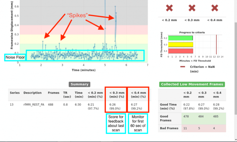
You can see an example of the output in the image below. The blue line is a running trace of what the estimated frame wise displacement is. This is the relative motion from frame to frame, combined over the 3 translation and 3 rotation directions. There is a shading:
- green: < 0.2 mm movement
- yellow: between 0.2 and 0.3 mm movement,
- red: between 0.3 and 0.4 mm movement
- grey: > 0.4mm movement
respective of total motion. These ranges are currently hard coded.
HCP uses some suggested metrics:
- Cancel the scan after the first 60sec if more than half of the initial frames have movements larger than 0.4mm (in the grey region).
- You can tell if this criteria is met by looking in the summary area, this updates in real-time.
- Part of the thinking behind this is that if they moved that much in the beginning, they most likely they also moved during the reference scans used in the SMS protocols, which can hurt the general quality of your entire run. Depending on your experiment, this may not be possible.
- Give your participant feedback. When the run completes, you will get summary statistics in the bottom summary panel. If less than 75% of the frames have movement less than .3mm, this is considered a ‘High Motion’ run. Feel free to determine your own thresholds and terminology for your participants, just be consistent.
How do I check my data for movement, ghosting, and spiking at the scanner?
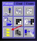
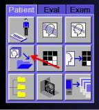
After every BOLD run you should scroll through your slices and look for movement, changes in ghosting, or changes in background luminance which could be spiking or RF interference. To do this, click on the Viewing tab on the far right side of the screen. In this window, you should load your BOLD images. Do this by bringing up the patient browser window by clicking on the image of the yellow folders in the lower right panel:
Navigate to your subject (newer sessions are towards the top, so the participant you are currently scanning should be the top-most directory) and then double click on the BOLD run you want to view, or drag it from the browser into the viewing window.
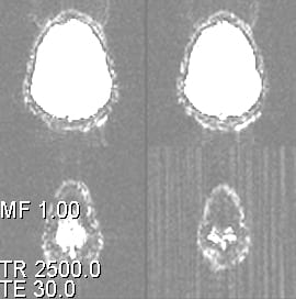
Next, you want to increase the background contrast to make it easier to see the ghosting and background noise. Do this by holding the middle button on the mouse and moving the mouse down and to the left. You want them to look something like the image below.
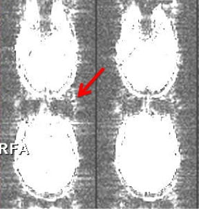
Once you have the contrast turned up, you should be able to see some ghosting (red arrow), which is normal. You want to make sure this doesn’t change much as you scroll through the images (by clicking on the up and down arrows on the right). In addition, you can look for changes in the background (the space outside of the brain). Sometimes you will see stripes appear (see image below). This is often a sign of RF interference or scanner spiking. You should also keep an eye on movement as you scroll through the images. See the image below for an example of what RF interference looks like. Please see here for what to do if something looks abnormal.
When you are done, please close the loaded images. This way the next users won’t see them, and the computer won’t become overloaded, which can happen if you load too many images at once. Do this by clicking on the close patient icon shown below.
What do I do if I find problems?
There are several basic steps you can do to try and improve the quality of your data at the scanner.
- Movement:
- Provide feedback to your subject about their movement, if your paradigm permits.
- In general, it can be useful to provide gentle reminders that they need to stay still, or you can specifically tell them that you checked their movement and you noticed that they moved at a particular time (such as, the beginning, middle, or end of scan). This can allow the subject to realize what kind of movements aren’t allowed.
- Note that if you are studying emotions, or working with a group of participants that might not respond well to this feedback, then you may want to consider saying nothing or providing very general, generic feedback.
- Ghosting:
- There is generally not a great solution for this. However, if you see sever ghosting or a change in ghosting across the run, Ross (rmair@fas.harvard.edu) should be informed of the date, subject number, and run number where something was observed.
- RF/Spiking:
- One common source of RF interference is the button box. Make sure the subject is holding the box down by their side and not up in the scanner bore near their head, and make sure they are keeping it stationary.
- This should also be reported to Ross (rmair@fas.harvard.edu) with the date, subject number, and run number where observed.
How do I check for correct coverage on my scans?
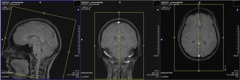
It is important to make sure that every part of the brain you want to collect information about is inside the field of view (yellow box).
Structural
For the structural, this means making sure the top, bottom, and sides of the brain are in the yellow box, and that the nose isn’t being cut off. Anything that falls just outside of the yellow FOV will ‘wrap around’ to the other side. For example, the noise would show up in the occipital lobe. If you use autoalign, then this will usually come up correctly for you, but it is always wise to look closely.
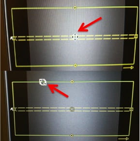
If you need to move the box, put your cursor over the center yellow circle, and your cursor will turn into the symbol shown below. To rotate the FOV, move the cursor to the edge of the box until you get the double arrows shown below. If you move the box in any other way, you will change the FOV. This is bad, as it can do things like change the voxel size.
Functional
For the functionals, setting the FOV (yellow box) is more complicated because it depends on the area of the brain you are interested in for your study. There is a trade off between voxel size, number of slices, and TR, so often you don’t have as many slices as necessary to cover all of the brain you want. If you are lucky enough to have plenty of slices and use autoalign, then you might not have to do anything. Regardless, you should visually check that the yellow box covers all the ‘important’ parts of the brain. This can be done by loading the structural scan up and looking at your slices on top of it. See step 4 (structural scan) of conducting a typical scan for more details on this.
If your FOV is small and you are worried about getting everything, you might want to run a test scan, with just 2 or 3 TRs to see what your actual BOLD images look like. See here for how to change the number of timepoints.
If you do need to move the FOV, you will have to copy this new position to all other subsequent scans that should be using the same slice prescription (other BOLDS, or fieldmap). Please see here for how to move your slices after autoalign doesn’t work.